【2023年】第31天 Logistic Regression with TensorFlow 2.0（用TensorFlow进行逻辑回归）

Logistic regression is one of the most popular classification methods.
Logistic回归是最流行的分类方法之一。
Although the name contains regression, and the underlying method is the same as that for linear regression, it is not a regression method.
虽然名字中含有回归，而且基本方法与线性回归的方法相同，但它不是一种回归方法。
That is, it is not used for prediction of continuous (numeric) values.
也就是说，它不用于预测连续（数字）值。
The purpose of the logistic regression method is to predict the outcome, which is categorical.
逻辑回归法的目的是预测结果，而结果是分类的。
As mentioned, logistic regression’s underlying method is the same as that for linear regression.
如前所述，逻辑回归的基本方法与线性回归的方法相同。
Suppose we take the multi-class linear equation, as shown following:
假设我们采取多类线性方程，如下所示：
y = m₁X₁ + m₂X₂ + m₃X₃ + …+m_nX_n + b
where x₁, x₂, x₃, …, x_n are different input features, m₁, m₂, m₃, … m_n are the slopes for different features, and b is the intercept.
其中x 表示的是不同的输入特征，m表示的是不同特征的斜率，b是截距。
We will apply a logistic function to the linear equation, as follows:
我们将对线性方程应用一个逻辑函数，如下所示：
p(y=1) = 1/(1 + e ^{-(m₁X₁ + m₂X₂ + m₃X₃ + …+m_nX_n + b)})
where p(y=1) is the probability value of y=1.
其中p(y=1)是y=1的概率值。
If we plot this function, it will look like an S, hence it is called a sigmoid function.
如果我们绘制这个函数，它看起来就像一个S，因此它被称为sigmoid函数。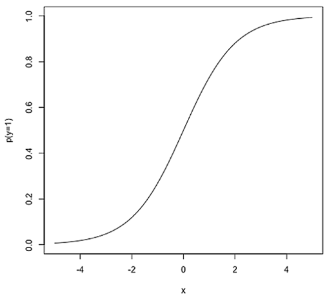

We will implement the logistic regression method in TensorFlow 2.0, using the iris data set and the LinearClassifier estimator available within the TensorFlow package.
我们将在TensorFlow 2.0中实现逻辑回归方法，使用虹膜数据集和TensorFlow软件包中的LinearClassifier估计器。

1. Import the required Modules

from __future__ import absolute_import, division, print_function, unicode_literals

import pandas as pd
import seaborn as sb
import tensorflow as tf
from tensorflow import keras
from tensorflow.estimator import LinearClassifier
from sklearn.model_selection import train_test_split
from sklearn.metrics import accuracy_score, precision_score, recall_score

print(tf.__version__)

2. Load and configure the Iris Dataset

col_names = ['SepalLength', 'SepalWidth', 'PetalLength', 'PetalWidth', 'Species']
target_dimensions = ['Setosa', 'Versicolor', 'Virginica']

training_data_path = tf.keras.utils.get_file("iris_training.csv", "https://storage.googleapis.com/download.tensorflow.org/data/iris_training.csv")
test_data_path = tf.keras.utils.get_file("iris_test.csv", "https://storage.googleapis.com/download.tensorflow.org/data/iris_test.csv")

training = pd.read_csv(training_data_path, names=col_names, header=0)
training = training[training['Species'] >= 1]
training['Species'] = training['Species'].replace([1,2], [0,1])
test = pd.read_csv(test_data_path, names=col_names, header=0)
test = test[test['Species'] >= 1]
test['Species'] = test['Species'].replace([1,2], [0,1])

training.reset_index(drop=True, inplace=True)
test.reset_index(drop=True, inplace=True)

iris_dataset = pd.concat([training, test], axis=0)

First, a list col_names is defined containing the names of the columns in the dataset: SepalLength, SepalWidth, PetalLength, PetalWidth and Species. where the first four columns are the characteristics (calyx length, calyx width, petal length and petal width) and the last column Species is the the target variable (species of iris).
首先，定义了一个列表col_names，包含了数据集中的列名：SepalLength、SepalWidth、PetalLength、PetalWidth和Species。其中，前四个列是特征（花萼长度、花萼宽度、花瓣长度和花瓣宽度），最后一列Species是目标变量（鸢尾花的品种）。
Next, another list target_dimensions is defined, containing different values for the target variables: Setosa, Versicolor and Virginica.
接着，定义了另一个列表target_dimensions，包含了目标变量的不同取值：Setosa、Versicolor和Virginica。
The training and test datasets are then downloaded from the specified URL by calling the tf.keras.utils.get_file() method and saved to the file paths specified by training_data_path and test_data_path respectively.
然后，通过调用tf.keras.utils.get_file()方法从指定的URL下载训练数据集和测试数据集，并分别保存到training_data_path和test_data_path指定的文件路径。
Next, use the pd.read_csv() method to read the CSV files of the training and test datasets and specify the column names as col_names, skipping the first row of the file as the column names.
接下来，使用pd.read_csv()方法读取训练数据集和测试数据集的CSV文件，并指定列名为col_names，跳过文件的第一行作为列名。
对于训练数据集，执行以下操作：

1. 保留Species列中取值大于等于1的行，即去除了原始数据集中Species取值为0的样本。
2. 将Species列中取值为1和2的样本替换为0和1，通过replace()方法实现。
   对于测试数据集，执行与训练数据集类似的操作。
   最后，使用pd.concat()方法将处理好的训练数据集和测试数据集按行堆叠在一起，得到完整的鸢尾花数据集iris_dataset。
   最后两行代码使用reset_index()方法重置了数据集的索引，使索引从零开始，并且通过设置drop=True丢弃原来的索引列。这样做是为了确保数据集索引的连续性。

iris_dataset.describe()

上述代码是在对名为"iris_dataset"的数据集进行描述性统计分析。通常，"describe()"是一个Pandas库中DataFrame对象的方法。
具体解释如下：

1. "iris_dataset"是一个数据集对象，可能是通过Pandas库中的read_csv()函数从CSV文件加载得到的，或者是从其他数据源获取的。这个数据集通常用于机器学习和数据分析领域。
2. ".describe()"是对数据集应用的方法，它会计算数据集中数值列的统计摘要信息。这些统计指标包括：计数（count）、均值（mean）、标准差（std）、最小值（min）、25%分位数（25%）、50%分位数（50%）、75%分位数（75%）和最大值（max）。
3. 该方法返回一个包含统计结果的DataFrame对象，其中每一列代表一个统计指标，每一行代表数据集中的一个数值列。
   总之，通过调用"iris_dataset.describe()"，你可以获得关于"iris_dataset"数据集中数值列的基本统计信息，以便更好地了解数据的分布和特征。
   Checking the relation between the variables using Pairplot and Correlation Graph
   使用配对图和相关图检查变量之间的关系

sb.pairplot(iris_dataset, diag_kind="kde")

运行结果：

这段代码是使用Seaborn库中的pairplot()函数来绘制一个数据集的散点图矩阵。在这个例子中，数据集被命名为iris_dataset。
pairplot()函数用于可视化多个变量之间的关系。它创建了一个网格，其中每个变量都与其他变量进行配对，并在对应的轴上绘制散点图或直方图。
pairplot()函数的第一个参数是要绘制的数据集iris_dataset。
第二个参数diag_kind="kde"指定对角线上的图形类型为核密度估计（Kernel Density Estimate，简称KDE）。
核密度估计是一种用于估计概率密度函数的非参数方法，通过平滑的曲线表示变量的分布情况。
生成一个散点图矩阵，其中包含iris_dataset数据集中各个变量之间的关系，并在对角线上显示每个变量的核密度估计图。

correlation_data = iris_dataset.corr()
correlation_data.style.background_gradient(cmap='coolwarm', axis=None)

运行结果：

上述代码是基于一个名为"iris_dataset"的数据集计算相关系数矩阵：

1. correlation_data = iris_dataset.corr() 这行代码计算了iris_dataset中各个特征（如花萼长度、花萼宽度等）之间的相关系数。相关系数是用来衡量两个变量之间线性关系强度的统计量，取值范围从-1到1。相关系数越接近1或-1表示两个变量之间具有较强的正相关或负相关关系，而接近0则表示无线性关系。
2. correlation_data.style.background_gradient(cmap=‘coolwarm’, axis=None) 这行代码将相关系数矩阵进行可视化，并应用了背景渐变效果。background_gradient() 方法根据相关系数的值来添加颜色映射，使得低相关性和高相关性的单元格具有不同的颜色。参数cmap='coolwarm’指定了使用"coolwarm"颜色映射，其中冷色调代表负相关性，暖色调代表正相关性。axis=None参数表示将整个矩阵应用渐变，而不是为每一行或列应用渐变。
   Descriptive Statistics - Central Tendency and Dispersion
   描述性统计 - 中心趋势和分散性

stats = iris_dataset.describe()
iris_stats = stats.transpose()
iris_stats

运行结果：

3. 使用describe()函数计算鸢尾花数据集（iris_dataset）的统计信息，并将结果赋值给变量stats。describe()函数会计算数据集中每个数值列的统计摘要，包括计数、均值、标准差、最小值、25%、50%和75%的分位数以及最大值。
4. 使用transpose()函数将stats中的统计信息转置，以便更好地展示和阅读。transpose()函数会交换数据框（DataFrame）的行和列。
Select the required columns
选择所需的列

X_data = iris_dataset[[m for m in iris_dataset.columns if m not in ['Species']]]
Y_data = iris_dataset[['Species']]

5. [m for m in iris_dataset.columns if m not in [‘Species’]] 用于生成一个列表，其中包含了所有不是 Species 的列名。这个列表作为索引，可以从 iris_dataset 中选出所有除了 Species 外的列。这些列组成的数据集被赋值给 X_data。
6. iris_dataset[[‘Species’]] 选出了 Species 列并将其转化为一个数据集，这个数据集被赋值给 Y_data。
7. X_data 包含了所有输入特征，而 Y_data 包含了目标变量 Species。
   Train Test Split
   训练测试分割

training_features , test_features ,training_labels, test_labels = train_test_split(X_data , Y_data , test_size=0.2)

1. 使用 train_test_split 函数，将数据集 X_data 和 Y_data 划分为训练集和测试集。
2. 具体来说，train_test_split 函数将数据集 X_data 和 Y_data 分别划分为训练集和测试集，其中 test_size=0.2 表示测试集所占比例为 20%。即将 80% 的数据作为训练数据，20% 的数据作为测试数据。
3. 函数的返回值是四个变量，分别为 training_features、test_features、training_labels 和 test_labels。
4. 其中，training_features 和 test_features 分别是训练集和测试集的输入特征，training_labels 和 test_labels 分别是训练集和测试集的目标变量。
   这段代码的作用是将数据集划分为训练集和测试集，并将划分后的训练集和测试集的输入特征和目标变量分别存储在变量 training_features、test_features、training_labels 和 test_labels 中，以便进行模型训练和测试。

print('No. of rows in Training Features: ', training_features.shape[0])
print('No. of rows in Test Features: ', test_features.shape[0])
print('No. of columns in Training Features: ', training_features.shape[1])
print('No. of columns in Test Features: ', test_features.shape[1])

print('No. of rows in Training Label: ', training_labels.shape[0])
print('No. of rows in Test Label: ', test_labels.shape[0])
print('No. of columns in Training Label: ', training_labels.shape[1])
print('No. of columns in Test Label: ', test_labels.shape[1])

运行结果：

1. training_features.shape[0] 和 test_features.shape[0] 分别输出训练集和测试集的行数，即样本数。
2. training_features.shape[1] 和 test_features.shape[1] 分别输出训练集和测试集的列数，即特征数。
3. training_labels.shape[0] 和 test_labels.shape[0] 分别输出训练集和测试集的行数，即样本数。
4. 由于目标变量只有一列，因此 training_labels.shape[1] 和 test_labels.shape[1] 都输出 1，即列数为 1。
5. 输出训练集和测试集的样本数和特征数，以及训练集和测试集的目标变量的样本数。

stats = training_features.describe()
stats = stats.transpose()
stats

运行结果：

1. 首先，describe() 函数用于计算训练集中每列数据的统计指标，包括计数（count）、均值（mean）、标准差（std）、最小值（min）、25% 分位数（25%）、50% 分位数（50%）、75% 分位数（75%）和最大值（max）。计算结果被赋值给变量 stats。
2. transpose() 函数被用于将 stats 的行和列交换，即将每列的统计指标转化为行，每行的特征名称转化为列。这么做的目的是为了方便查看每个特征的统计指标。

stats = test_features.describe()
stats = stats.transpose()
stats

运行结果：

1. describe() 函数用于计算测试集中每列数据的统计指标，包括计数（count）、均值（mean）、标准差（std）、最小值（min）、25% 分位数（25%）、50% 分位数（50%）、75% 分位数（75%）和最大值（max）。计算结果被赋值给变量 stats。
2. transpose() 函数被用于将 stats 的行和列交换，即将每列的统计指标转化为行，每行的特征名称转化为列。这么做的目的是为了方便查看每个特征的统计指标。
   Normalize Data
   归一化数据

def norm(x):
  stats = x.describe()
  stats = stats.transpose()
  return (x - stats['mean']) / stats['std']

normed_train_features = norm(training_features)
normed_test_features = norm(test_features)

1. 这段代码定义了一个名为 norm 的函数，并使用该函数对训练集和测试集的输入特征进行标准化处理。
2. norm 函数的作用是对输入的数据进行标准化处理。具体来说，它先计算出数据集中每个特征的均值和标准差，并将这些统计指标保存在 stats 中。
3. 通过将数据集中每个特征减去该特征的均值，再除以该特征的标准差，将数据集中每个特征标准化到均值为 0，标准差为 1 的范围内。最后返回标准化后的数据集。
4. normed_train_features 和 normed_test_features 分别接收 norm 函数处理后的训练集和测试集的输入特征。这样做的目的是将数据集中的每个特征标准化，以便于模型训练和测试。

Build the Input Pipeline for TensorFlow model
为TensorFlow模型建立输入管道

def feed_input(features_dataframe, target_dataframe, num_of_epochs=10, shuffle=True, batch_size=32):
  def input_feed_function():
    dataset = tf.data.Dataset.from_tensor_slices((dict(features_dataframe), target_dataframe))
    if shuffle:
      dataset = dataset.shuffle(2000)
    dataset = dataset.batch(batch_size).repeat(num_of_epochs)
    return dataset
  return input_feed_function

train_feed_input = feed_input(normed_train_features, training_labels)
train_feed_input_testing = feed_input(normed_train_features, training_labels, num_of_epochs=1, shuffle=False)
test_feed_input = feed_input(normed_test_features, test_labels, num_of_epochs=1, shuffle=False)

1. feed_input(features_dataframe, target_dataframe, num_of_epochs=10, shuffle=True, batch_size=32)：这是一个函数定义，它接受特征数据和目标数据作为输入，并可选地指定训练的 epochs 数量、是否打乱数据以及批处理大小。
2. def input_feed_function():：这是内部定义的一个辅助函数，用于创建数据集。
3. dataset = tf.data.Dataset.from_tensor_slices((dict(features_dataframe), target_dataframe))：将特征数据和目标数据转换为 TensorFlow 的数据集。from_tensor_slices() 函数将每个样本的特征和目标作为元组切片，并创建一个数据集。
4. if shuffle: dataset = dataset.shuffle(2000)：如果设置了 shuffle 为 True，则对数据集进行洗牌操作。shuffle() 函数将数据集中的元素随机打乱。
5. dataset = dataset.batch(batch_size).repeat(num_of_epochs)：将数据集按照指定的批处理大小进行分批，并重复多个 epochs。batch() 函数将数据集分成批次，每个批次包含指定数量的样本。repeat() 函数将数据集重复多个 epochs，以便在训练过程中多次使用相同的数据。
6. return dataset：返回创建的数据集。
7. return input_feed_function：返回辅助函数 input_feed_function 的引用。这意味着可以使用 train_feed_input = feed_input(normed_train_features, training_labels) 来调用 feed_input 函数，并将返回的函数对象赋值给 train_feed_input。
8. train_feed_input = feed_input(normed_train_features, training_labels)：调用 feed_input 函数，传入规范化后的训练特征数据和训练标签数据。这将返回一个用于训练的数据集。
9. train_feed_input_testing = feed_input(normed_train_features, training_labels, num_of_epochs=1, shuffle=False)：调用 feed_input 函数，并指定仅进行 1 个 epoch 的训练，并且不打乱数据。这将返回一个用于测试的数据集。
   10.test_feed_input = feed_input(normed_test_features, test_labels, num_of_epochs=1, shuffle=False)：调用 feed_input 函数，并指定仅进行 1 个 epoch 的训练，并且不打乱数据。这将返回一个用于测试的数据集。
   总结起来，上述代码定义了一个用于数据输入的函数 feed_input，它将特征数据和目标数据转换为 TensorFlow 的数据集，并进行批处理和重复处理以用于模型的训练和测试。
   Model Training
   模型训练

feature_columns_numeric = [tf.feature_column.numeric_column(m) for m in training_features.columns]

1. feature_columns_numeric：这是一个变量名，用于存储数字列特征的列表。
2. tf.feature_column.numeric_column(m)：这是TensorFlow中的一个函数，用于创建一个表示数字特征的特征列。它接受一个参数 m，该参数是一个字符串，表示训练特征数据框中的一个列名。
3. for m in training_features.columns：这是一个循环语句，遍历了training_features数据框的所有列名。在每次迭代中，将当前列名赋值给变量 m。
4. [tf.feature_column.numeric_column(m) for m in training_features.columns]：这是一个列表推导式（list comprehension），它使用循环遍历数据框的每个列名，并将通过 tf.feature_column.numeric_column 函数创建的数字列特征添加到列表中。最终得到的列表包含了数据框中所有列的数字列特征。

logistic_model = LinearClassifier(feature_columns=feature_columns_numeric)

1. logistic_model：这是一个变量名，用于存储创建的逻辑回归模型。
2. LinearClassifier：这是TensorFlow中的一个类，用于创建线性分类器模型。它接受一个参数 feature_columns，该参数是包含特征列的列表，用于指定输入特征。
3. feature_columns=feature_columns_numeric：这是将数字列特征列表 feature_columns_numeric 分配给 feature_columns 参数的语法。通过此参数，我们告诉模型要使用哪些特征列作为输入。

1. logistic_model：这是之前创建的逻辑回归模型。
2. .train(train_feed_input)：这是调用逻辑回归模型对象的 train() 方法来执行模型的训练。该方法接受一个参数 train_feed_input，表示用于训练的输入数据。
3. train_feed_input：这是训练数据的输入。它可能是一个包含特征和标签的数据集对象，或者是一个字典或迭代器，提供了特征和标签之间的映射关系。
   Predictions
   预测

train_predictions = logistic_model.predict(train_feed_input_testing)
test_predictions = logistic_model.predict(test_feed_input)

1. logistic_model：这是之前训练好的逻辑回归模型。
2. .predict(train_feed_input_testing)：这是调用逻辑回归模型对象的 predict() 方法来进行预测。该方法接受一个参数 train_feed_input_testing，表示用于预测的输入数据。
3. train_feed_input_testing：这是训练集的输入数据，用于进行预测。
4. train_predictions：这是变量名，用于存储训练集的预测结果。
5. test_predictions：这是变量名，用于存储测试集的预测结果。

train_predictions_series = pd.Series([p['classes'][0].decode("utf-8")   for p in train_predictions])
test_predictions_series = pd.Series([p['classes'][0].decode("utf-8")   for p in test_predictions])

1. pd.Series()：这是 Pandas 库中的一个函数，用于创建 Series 对象，它是一种带有标签的一维数组。
2. [p[‘classes’][0].decode(“utf-8”) for p in train_predictions]：这是一个列表推导式（list comprehension），通过遍历 train_predictions 中的每个预测结果 p，提取其中的 ‘classes’ 键对应的值，并使用 decode(“utf-8”) 将其从字节码解码为字符串。最终得到的列表就是包含训练集预测结果的字符串列表。
3. [p[‘classes’][0].decode(“utf-8”) for p in test_predictions]：类似地，这也是一个列表推导式，通过遍历 test_predictions 中的每个预测结果 p，提取其中的 ‘classes’ 键对应的值，并解码为字符串。最终得到的列表就是包含测试集预测结果的字符串列表。
4. train_predictions_series：这是变量名，用于存储将训练集预测结果转换为 Series 对象后的结果。
5. test_predictions_series：这是变量名，用于存储将测试集预测结果转换为 Series 对象后的结果。

train_predictions_df = pd.DataFrame(train_predictions_series, columns=['predictions'])
test_predictions_df = pd.DataFrame(test_predictions_series, columns=['predictions'])

1. pd.DataFrame() 是 Pandas 库中用于创建数据帧的函数。
2. train_predictions_series 是包含训练预测数据的序列对象。
3. columns=[‘predictions’] 指定了数据帧的列名。在这种情况下，数据帧将有一个名为 ‘predictions’ 的列。
4. 创建的数据帧被赋值给变量 train_predictions_df。
5. 类似地，此行使用 test_predictions_series 创建另一个数据帧。
6. 它与前一行具有相同的结构，创建一个名为 ‘predictions’ 的单列数据帧。
7. 创建的数据帧被赋值给变量 test_predictions_df。

training_labels.reset_index(drop=True, inplace=True)
train_predictions_df.reset_index(drop=True, inplace=True)

test_labels.reset_index(drop=True, inplace=True)
test_predictions_df.reset_index(drop=True, inplace=True)

1. training_labels.reset_index(drop=True, inplace=True) 这行代码针对名为 training_labels 的 DataFrame 执行了重置索引操作。传递参数 drop=True 表示丢弃原有的索引，并将重新生成的索引替换原有的索引。inplace=True 参数表示在原地进行修改，即直接修改原始的 DataFrame，而不是创建一个新的副本。
2. train_predictions_df.reset_index(drop=True, inplace=True)
   类似地，这行代码对名为 train_predictions_df 的 DataFrame 执行了重置索引操作。同样，指定 drop=True 参数会丢弃原有的索引，并用重新生成的索引替代。inplace=True 则表示直接在原 DataFrame 上进行修改。
3. test_labels.reset_index(drop=True, inplace=True)
   这行代码对名为 test_labels 的 DataFrame 进行了重置索引操作。通过指定 drop=True 参数，它丢弃了原有的索引，并使用重新生成的索引取而代之。inplace=True 表示直接在原 DataFrame 上进行修改。
4. test_predictions_df.reset_index(drop=True, inplace=True)
   最后一行代码重置了 test_predictions_df 的索引。与前面的例子类似，drop=True 参数会丢弃原有的索引，并使用重新生成的索引代替。inplace=True 则表示直接在原有 DataFrame 上进行修改。

train_labels_with_predictions_df = pd.concat([training_labels, train_predictions_df], axis=1)
test_labels_with_predictions_df = pd.concat([test_labels, test_predictions_df], axis=1)

1. 使用 Pandas 的 concat() 函数将两个 DataFrame 进行列方向的合并。
2. train_labels_with_predictions_df = pd.concat([training_labels, train_predictions_df], axis=1)
   这行代码创建了一个名为 train_labels_with_predictions_df 的新 DataFrame。它通过 pd.concat() 函数将 training_labels 和 train_predictions_df 两个 DataFrame 按列方向（即轴标识符 axis=1）进行合并。
3. test_labels_with_predictions_df = pd.concat([test_labels, test_predictions_df], axis=1)
   类似地，这行代码创建了一个名为 test_labels_with_predictions_df 的新 DataFrame。它也是通过 pd.concat() 函数将 test_labels 和 test_predictions_df 两个 DataFrame 按列方向进行合并。
   Validation
   验证

def calculate_binary_class_scores(y_true, y_pred):
  accuracy = accuracy_score(y_true, y_pred.astype('int64'))
  precision = precision_score(y_true, y_pred.astype('int64'))
  recall = recall_score(y_true, y_pred.astype('int64'))
  return accuracy, precision, recall

1. 定义了一个名为 calculate_binary_class_scores 的函数，该函数接受两个参数 y_true 和 y_pred，表示真实标签和预测标签。
2. accuracy = accuracy_score(y_true, y_pred.astype(‘int64’))
   这行代码使用 accuracy_score 函数计算分类准确率。accuracy_score 函数接受真实标签 (y_true) 和预测标签 (y_pred) 作为输入，并返回分类准确率。在这里，为了保证数据类型一致性，通过 astype(‘int64’) 将预测标签转换为整数类型。
3. precision = precision_score(y_true, y_pred.astype(‘int64’))
   类似地，这行代码使用 precision_score 函数计算精确度（Precision）。precision_score 函数接受真实标签和预测标签作为输入，并返回精确度。同样地，为了保证数据类型一致性，将预测标签转换为整数类型。
4. recall = recall_score(y_true, y_pred.astype(‘int64’))
   这行代码使用 recall_score 函数计算召回率（Recall）。recall_score 函数接受真实标签和预测标签作为输入，并返回召回率。同样地，为了保证数据类型一致性，将预测标签转换为整数类型。
5. return accuracy, precision, recall
   最后一行代码使用 return 语句返回计算得到的分类准确率、精确度和召回率作为函数的输出。

train_accuracy_score, train_precision_score, train_recall_score = calculate_binary_class_scores(training_labels, train_predictions_series)
test_accuracy_score, test_precision_score, test_recall_score = calculate_binary_class_scores(test_labels, test_predictions_series)

print('Training Data Accuracy (%) = ', round(train_accuracy_score*100,2))
print('Training Data Precision (%) = ', round(train_precision_score*100,2))
print('Training Data Recall (%) = ', round(train_recall_score*100,2))
print('-'*50)
print('Test Data Accuracy (%) = ', round(test_accuracy_score*100,2))
print('Test Data Precision (%) = ', round(test_precision_score*100,2))
print('Test Data Recall (%) = ', round(test_recall_score*100,2))

运行结果：

1. calculate_binary_class_scores 函数计算训练数据和测试数据的分类准确率、精确度和召回率，并打印这些评估指标的结果。
2. train_accuracy_score, train_precision_score, train_recall_score = calculate_binary_class_scores(training_labels, train_predictions_series)
   这行代码调用 calculate_binary_class_scores 函数，传入训练数据的真实标签 (training_labels) 和预测标签 (train_predictions_series)。返回的三个评估指标（分类准确率、精确度、召回率）分别赋值给变量 train_accuracy_score、train_precision_score 和 train_recall_score。
3. test_accuracy_score, test_precision_score, test_recall_score = calculate_binary_class_scores(test_labels, test_predictions_series)
   类似地，这行代码调用 calculate_binary_class_scores 函数，传入测试数据的真实标签 (test_labels) 和预测标签 (test_predictions_series)。返回的三个评估指标赋值给变量 test_accuracy_score、test_precision_score 和 test_recall_score。
4. print('Training Data Accuracy (%) = ', round(train_accuracy_score*100,2))
   这行代码打印训练数据的分类准确率。通过将 train_accuracy_score 乘以 100 并取两位小数，使用 round() 函数对结果进行四舍五入。
5. print('Training Data Precision (%) = ', round(train_precision_score*100,2))
   类似地，这行代码打印训练数据的精确度。
6. print('Training Data Recall (%) = ', round(train_recall_score*100,2))
   这行代码打印训练数据的召回率。
7. print(’-’*50)
   这行代码打印分隔线，用于区分训练数据和测试数据的评估结果。
8. print('Test Data Accuracy (%) = ', round(test_accuracy_score*100,2))
   这行代码打印测试数据的分类准确率。
9. print('Test Data Precision (%) = ', round(test_precision_score*100,2))
   类似地，这行代码打印测试数据的精确度。
10. print('Test Data Recall (%) = ', round(test_recall_score*100,2))
    这行代码打印测试数据的召回率。