【2023年】第32天 Boosted Trees with TensorFlow 2.0（随机森林）

一、Ensemble Technique 集合技术
An ensemble is a collection of predictors. For example, instead of using a single model (say, logistic regression) for a classification problem, we can use multiple models (say, logistic regression + decision trees, etc.) to perform predictions.
集合是一个预测器的集合。
例如，我们可以使用多个模型（如逻辑回归+决策树等）来进行预测，而不是使用单一模型（如逻辑回归）来处理分类问题。
The outputs from the predictors are combined by different averaging methods, such as weighted averages, normal averages, or votes, and a final prediction value is derived. Ensemble methods have been proved to be more effective than individual methods and, therefore, are heavily used to build machine learning models.
预测器的输出通过不同的平均方法进行组合，如加权平均、正常平均或投票，并得出最终预测值。集合方法已被证明比单个方法更有效，因此，被大量用于建立机器学习模型。
Ensemble methods can be implemented by either bagging or boosting.
集成方法可以通过 bagging 或 boosting 来实现。
二、Bagging
Bagging和Boosting的区别
Bagging：训练集是在原始集中有放回选取的，从原始集中选出的各轮训练集之间是独立的。
Boosting：每一轮的训练集不变，只是训练集中每个样例在分类器中的权重发生变化。 而权值是根据上一轮的分类结果进行调整。 Boosting：根据错误率不断调整样例的权值，错误率越大则权重越大。
Bagging is a technique wherein we build independent models/predictors, using a random subsample/bootstrap of data for each of the models/predictors.
Bagging是一种技术，我们建立独立的模型/预测器，对每个模型/预测器使用随机的子样本/bootstrap数据。
Then an average (weighted, normal, or by voting) of the scores from the different predictors is taken to get the final score/prediction.
然后对不同预测器的分数进行平均（加权、正常或投票），得到最终的分数/预测。
The most famous bagging method is random forest.
最著名的Bagging方法是随机森林。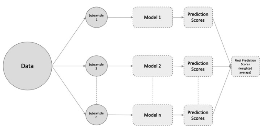

三、Boosting
Boosting is a different ensemble technique, wherein the predictors are not independently trained but done so in a sequential manner.
Boosting是一种不同的集合技术，其中预测器不是独立训练的，而是以连续的方式进行的。
For example, we build a logistic regression model on a subsample/bootstrap of the original training data set.
例如，我们在原始训练数据集的一个子样本/bootstrap上建立一个逻辑回归模型。
Then we take the output of this model and feed it to a decision tree, to get the prediction, and so on.
然后，我们把这个模型的输出送入一个决策树，得到预测结果，如此反复。
The aim of this sequential training is for the subsequent models to learn from the mistakes of the previous model.
这种顺序训练的目的是让后面的模型从前面模型的错误中学习。
Gradient boosting is an example of a boosting method.
梯度提升是提升方法的一个例子。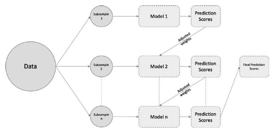

四、Gradient Boosting
The main difference between gradient boosting compared to other boosting methods is that instead of incrementing the weights of misclassified outcomes from one previous learner to the next, we optimize the loss function of the previous learner.
与其他提升方法相比，梯度提升的主要区别在于，我们不是将错误分类的结果的权重从之前的学习者增加到下一个学习者，而是优化之前学习者的损失函数。
We will be building a boosted trees classifier, using the gradient boosting method under the hood.
我们将建立一个升压树分类器，在引擎盖下使用梯度升压方法。
We will take the iris data set for classification.
我们将使用鸢尾花数据集进行分类。
As we have already used the same data set for implementing logistic regression in the previous section, we will keep the preprocessing the same (i.e., until the “Build the input pipeline for TensorFlow model” step from the previous example).
由于我们已经在上一节中使用了相同的数据集来实现逻辑回归，我们将保持预处理的方式不变（即直到上一例中的 "为TensorFlow模型建立输入管道 "步骤）。
We will continue directly with the model training step, as follows:
我们将直接继续进行模型训练步骤，如下所示：

1. Import the required Modules
   导入所需的模块

from __future__ import absolute_import, division, print_function, unicode_literals

import numpy as np
import pandas as pd
import seaborn as sb
import tensorflow as tf
from tensorflow import keras
from sklearn.model_selection import train_test_split
from sklearn.metrics import accuracy_score, precision_score, recall_score

print(tf.__version__)

2. Load and configure the Iris Dataset
   加载并配置鸢尾花数据集。

CSV_COLUMN_NAMES = ['SepalLength', 'SepalWidth', 'PetalLength', 'PetalWidth', 'Species']
SPECIES = ['Setosa', 'Versicolor', 'Virginica']

train_path = tf.keras.utils.get_file("iris_training.csv", "https://storage.googleapis.com/download.tensorflow.org/data/iris_training.csv")
test_path = tf.keras.utils.get_file("iris_test.csv", "https://storage.googleapis.com/download.tensorflow.org/data/iris_test.csv")

train = pd.read_csv(train_path, names=CSV_COLUMN_NAMES, header=0)
train = train[train.Species >= 1]
train['Species'] = train['Species'].replace([1,2], [0,1])
test = pd.read_csv(test_path, names=CSV_COLUMN_NAMES, header=0)
test = test[test.Species >= 1]
test['Species'] = test['Species'].replace([1,2], [0,1])

train.reset_index(drop=True, inplace=True)
test.reset_index(drop=True, inplace=True)

iris_dataset = pd.concat([train, test], axis=0)

1. CSV_COLUMN_NAMES：定义了CSV文件中的列名称，包括’SepalLength’、‘SepalWidth’、‘PetalLength’、‘PetalWidth’和’Species’。
2. SPECIES：定义了鸢尾花的三个品种，分别为’Setosa’、‘Versicolor’和’Virginica’。
3. train_path和test_path：使用tf.keras.utils.get_file函数从指定的URL下载训练集和测试集的CSV文件，并返回本地保存的文件路径。
4. train和test：使用pd.read_csv函数读取CSV文件，并根据给定的列名（names=CSV_COLUMN_NAMES）和标题行位置（header=0）创建数据帧（DataFrame）。然后通过筛选操作，仅保留Species大于等于1的样本。
5. train[‘Species’] = train[‘Species’].replace([1,2], [0,1])和test[‘Species’] = test[‘Species’].replace([1,2], [0,1])：将训练集和测试集中的标签值进行替换，将原来的类别1和2分别映射为0和1，以便进行二分类任务。
6. train.reset_index(drop=True, inplace=True)和test.reset_index(drop=True, inplace=True)：重置训练集和测试集的索引，去除原始索引并按顺序重新分配索引值。
7. iris_dataset = pd.concat([train, test], axis=0)：将处理过的训练集和测试集按照行方向（axis=0）进行合并，得到最终的鸢尾花数据集（iris_dataset）。

iris_dataset.describe()

运行结果：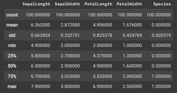

1. 上述代码是在使用iris_dataset数据集的describe()方法。describe()是一个用于描述统计信息的函数，它提供了关于数据集中每个数值列的统计摘要。
2. 通常情况下，iris_dataset是一个包含鸢尾花数据的数据集对象。通过调用describe()方法，可以获取有关该数据集的各种统计信息。
3. 计数（Count）：显示每个数值列中非缺失值的观测数量。
4. 平均值（Mean）：表示每个数值列的平均值。
5. 标准差（Standard Deviation）：用于衡量每个数值列中数据点的离散程度。
6. 最小值（Minimum）：给出每个数值列的最小值。
7. 第25百分位数（25th percentile）：给出每个数值列的第25百分位数，也被称为第一四分位数。
8. 中位数（Median）：表示每个数值列的中位数，即将所有观测值排序后的中间值。
9. 第75百分位数（75th percentile）：给出每个数值列的第75百分位数，也被称为第三四分位数。
10. 最大值（Maximum）：给出每个数值列的最大值。
    Checking the relation between the variables using Pairplot and Correlation Graph
    使用配对图和相关图检查变量之间的关系

sb.pairplot(iris_dataset, diag_kind="kde")

运行结果：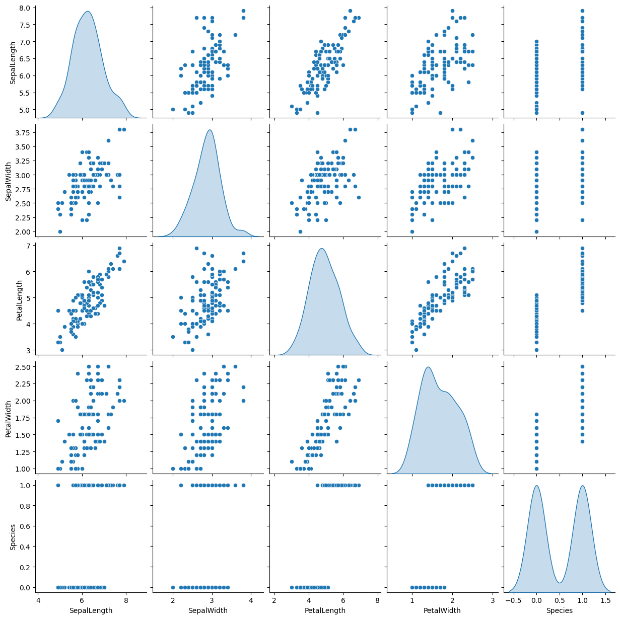

correlation_data = iris_dataset.corr()
correlation_data.style.background_gradient(cmap='coolwarm', axis=None)

运行结果：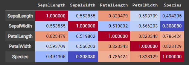

1. 针对鸢尾花数据集（iris_dataset）进行相关性分析的操作。首先，代码调用了corr()函数，该函数计算了整个数据集中各个特征之间的相关性。
2. 通过调用style.background_gradient()方法，将相关性结果可视化为一个渐变色的热力图。coolwarm颜色映射来表示相关性的程度。参数axis=None表示相关性热力图不会根据轴的不同而着色，而是整体呈现整个数据集的相关性情况。
   Descriptive Statistics - Central Tendency and Dispersion
   描述性统计 - 中心趋势和分散性

stats = iris_dataset.describe()
iris_stats = stats.transpose()
iris_stats

运行结果：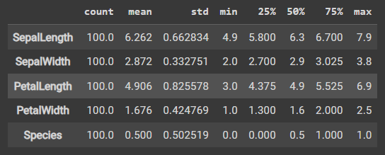

1. 针对鸢尾花数据集（iris dataset）进行描述性统计分析的操作。假设已经加载了鸢尾花数据集并将其存储在变量iris_dataset中。
2. stats = iris_dataset.describe(): 这一行代码使用describe()函数计算了鸢尾花数据集的描述统计信息，并将结果存储在stats变量中。描述统计信息包括计数（count）、均值（mean）、标准差（std）、最小值（min）、四分位数（25%、50%、75%）和最大值（max）。
3. iris_stats = stats.transpose(): 这一行代码对stats进行转置操作，即将统计结果的行列互换。转置后的结果存储在iris_stats变量中。通过转置，我们可以将不同特征（如花萼长度、花萼宽度等）的统计信息以列的形式进行展示，更加方便查看和分析。
   Select the required columns
   选择所需的列

X_data = iris_dataset[[i for i in iris_dataset.columns if i not in ['Species']]]
Y_data = iris_dataset[['Species']]

1. X_data 是一个包含除了 ‘Species’ 列以外的所有列的子集。列表推导式 [i for i in iris_dataset.columns if i not in [‘Species’]] 用来获取 iris_dataset 中不包含 ‘Species’ 的列名，并将这些列作为索引从 iris_dataset 提取出来，存储在 X_data 变量中。
2. Y_data 是一个包含 ‘Species’ 列的子集。这里使用双括号将 ‘Species’ 列名包裹起来，表示将其作为 DataFrame 列名提取出来，并将提取到的列赋值给 Y_data 变量。
   Train Test Split
   训练测试分割

train_features , test_features ,train_labels, test_labels = train_test_split(X_data , Y_data , test_size=0.3)

1. 使用 train_test_split 函数将数据集划分为训练集和测试集，并将划分后的特征和标签分别赋值给 train_features、test_features、train_labels 和 test_labels 变量。
2. X_data 是特征集，包含了所有特征列的数据。Y_data 是目标变量集，包含了标签列的数据。
3. train_test_split 函数用于将数据集划分为训练集和测试集。其中，test_size=0.3 表示将数据集中的 30% 分配给测试集，而剩余的 70% 分配给训练集。
4. 根据给定的参数，train_test_split(X_data, Y_data, test_size=0.3) 执行后会返回四个变量：
   train_features：训练集的特征数据，即划分后的 X_data 的训练集部分。
   test_features：测试集的特征数据，即划分后的 X_data 的测试集部分。
   train_labels：训练集的标签数据，即划分后的 Y_data 的训练集部分。
   test_labels：测试集的标签数据，即划分后的 Y_data 的测试集部分。

print('Training Features Rows: ', train_features.shape[0])
print('Test Features Rows: ', test_features.shape[0])
print('Training Features Columns: ', train_features.shape[1])
print('Test Features Columns: ', test_features.shape[1])

print('Training Label Rows: ', train_labels.shape[0])
print('Test Label Rows: ', test_labels.shape[0])
print('Training Label Columns: ', train_labels.shape[1])
print('Test Label Columns: ', test_labels.shape[1])

运行结果：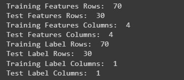

用于打印训练集和测试集的特征矩阵和标签矩阵的行数和列数。
（1）train_features.shape[0]：打印训练集特征矩阵的行数，即训练集中样本的数量。
（2）test_features.shape[0]：打印测试集特征矩阵的行数，即测试集中样本的数量。
（3）train_features.shape[1]：打印训练集特征矩阵的列数，即特征的数量。
（4）test_features.shape[1]：打印测试集特征矩阵的列数，即特征的数量。
（5）train_labels.shape[0]：打印训练集标签矩阵的行数，即训练集中样本的数量。
（6）test_labels.shape[0]：打印测试集标签矩阵的行数，即测试集中样本的数量。
（7）train_labels.shape[1]：打印训练集标签矩阵的列数，即标签的数量。
（8）test_labels.shape[1]：打印测试集标签矩阵的列数，即标签的数量。

stats = train_features.describe()
stats = stats.transpose()
stats

运行结果：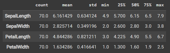

stats = test_features.describe()
stats = stats.transpose()
stats

运行结果：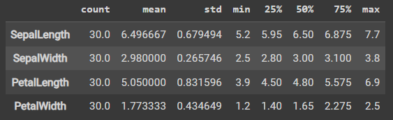

Normalize Data
归一化数据

def norm(x):
  stats = x.describe()
  stats = stats.transpose()
  return (x - stats['mean']) / stats['std']

normed_train_features = norm(train_features)
normed_test_features = norm(test_features)

1. 定义了一个名为 norm(x) 的函数，它接受一个输入 x 并使用 x 的均值和标准差对其进行归一化处理。
2. 在函数内部，通过调用 describe() 方法计算了 x 的统计信息，并将结果赋值给变量 stats。
3. 调用 transpose() 方法对 stats 进行转置操作，将行和列进行交换，以便更容易访问均值和标准差。
4. 表达式 (x - stats[‘mean’]) / stats[‘std’] 将 x 减去均值并除以标准差。这个公式用于对数据进行标准化处理，确保数据具有零均值和单位方差。
   Build the Input Pipeline for TensorFlow model
   为TensorFlow模型建立输入管道

def feed_input(features_df, target_df, num_of_epochs=10, shuffle=True, batch_size=35):
  def input_feed_function():
    dataset = tf.data.Dataset.from_tensor_slices((dict(features_df), target_df))
    if shuffle:
      dataset = dataset.shuffle(1000)
    dataset = dataset.batch(batch_size).repeat(num_of_epochs)
    return dataset
  return input_feed_function

train_feed_input = feed_input(normed_train_features, train_labels)
train_feed_input_testing = feed_input(normed_train_features, train_labels, num_of_epochs=1, shuffle=False)
test_feed_input = feed_input(normed_test_features, test_labels, num_of_epochs=1, shuffle=False)

1. 函数内部定义了一个嵌套函数input_feed_function()，它是一个输入数据的生成器函数。这个函数使用tf.data.Dataset.from_tensor_slices方法将特征数据集和目标数据集合并，并转换成tf.data.Dataset类型的数据集对象。
2. train_feed_input: 用于训练模型的数据集对象。它使用了normed_train_features作为特征数据集，train_labels作为目标数据集，默认使用了10个时期(epoch)，进行数据洗牌(shuffle)并以批次大小(batch_size)为35。
3. train_feed_input_testing: 用于测试训练模型的数据集对象。它与train_feed_input相同，但只使用了1个时期(epoch)，不进行数据洗牌(shuffle)。
4. test_feed_input: 用于测试模型性能的数据集对象。它使用了normed_test_features作为特征数据集，test_labels作为目标数据集，默认使用了1个时期(epoch)，且不进行数据洗牌(shuffle)。

feature_columns_numeric = [tf.feature_column.numeric_column(k) for k in train_features.columns]

1. 使用 TensorFlow（tf）的特征列（feature column）功能来创建数值特征的列表。
2. 代码的第一行使用一个列表推导式（list comprehension）遍历 train_features.columns 中的每个特征，并为每个特征创建一个数值特征列。tf.feature_column.numeric_column(k) 表示创建一个数值特征列，其中 k 是特征的名称。

rf_model = tf.estimator.BoostedTreesClassifier(feature_columns=feature_columns_numeric, n_batches_per_layer=1)

使用 TensorFlow（tf）中的 tf.estimator.BoostedTreesClassifier 函数创建了一个梯度提升树分类器模型（Boosted Trees Classifier）。

1. feature_columns=feature_columns_numeric：将之前创建的数值特征列列表 feature_columns_numeric 作为参数传递给模型。这些特征列将用作输入模型的特征。
2. n_batches_per_layer=1：此参数指定每层训练时使用的批次数量。在梯度提升树算法中，每个批次会计算一组决策树，并将其添加到集成中。通过设置 n_batches_per_layer=1，每层只使用一个批次，也就是每次迭代只构建一棵决策树。

rf_model.train(train_feed_input)

rf_model.train(train_feed_input) 表示对随机森林模型 rf_model 进行训练，其中 train_feed_input 是训练数据的输入。训练数据通常是一个特征矩阵和对应的目标变量（标签）组成的数据集，用于训练模型以学习特征与目标变量之间的关系。
Predictions
预测

train_predictions = rf_model.predict(train_feed_input_testing)
test_predictions = rf_model.predict(test_feed_input)

1. rf_model.predict(train_feed_input_testing) 表示使用训练好的随机森林模型 rf_model 对测试数据集 train_feed_input_testing 进行预测，并将预测结果存储在 train_predictions 中。
2. rf_model.predict(test_feed_input) 表示使用训练好的随机森林模型 rf_model 对另一个测试数据集 test_feed_input 进行预测，并将预测结果存储在 test_predictions 中。

train_predictions_series = pd.Series([p['classes'][0].decode("utf-8")   for p in train_predictions])
test_predictions_series = pd.Series([p['classes'][0].decode("utf-8")   for p in test_predictions])

1. pd.Series([p[‘classes’][0].decode(“utf-8”) for p in train_predictions]) 表示将训练数据集的预测结果 train_predictions 转换为一个 Pandas Series 对象，并存储在名为 train_predictions_series 的变量中。
2. 其中，p[‘classes’][0] 表示每个预测结果中的类别信息（通常是编码形式），通过 .decode(“utf-8”) 进行解码，将其转换为字符串类型。
3. pd.Series([p[‘classes’][0].decode(“utf-8”) for p in test_predictions]) 表示将测试数据集的预测结果 test_predictions 转换为另一个 Pandas Series 对象，并存储在名为 test_predictions_series 的变量中。

train_predictions_df = pd.DataFrame(train_predictions_series, columns=['predictions'])
test_predictions_df = pd.DataFrame(test_predictions_series, columns=['predictions'])

train_labels.reset_index(drop=True, inplace=True)
train_predictions_df.reset_index(drop=True, inplace=True)

test_labels.reset_index(drop=True, inplace=True)
test_predictions_df.reset_index(drop=True, inplace=True)

1. train_labels.reset_index(drop=True, inplace=True) 表示将训练数据集的标签 train_labels 的索引重置为默认的整数索引，并丢弃原来的索引。drop=True 参数表示丢弃原有的索引列，而不会将其保留为新的一列。inplace=True 参数表示直接在原始对象上进行操作，而不返回一个新的对象。
2. train_predictions_df.reset_index(drop=True, inplace=True) 表示将训练数据集的预测结果 DataFrame train_predictions_df 的索引重置为默认的整数索引，并丢弃原来的索引列。
3. test_labels.reset_index(drop=True, inplace=True) 和 test_predictions_df.reset_index(drop=True, inplace=True) 分别对测试数据集的标签和预测结果进行了相同的操作。

train_labels_with_predictions_df = pd.concat([train_labels, train_predictions_df], axis=1)
test_labels_with_predictions_df = pd.concat([test_labels, test_predictions_df], axis=1)

1. pd.concat([train_labels, train_predictions_df], axis=1) 表示使用 Pandas 的 concat 函数将训练数据集的标签 train_labels 和预测结果 DataFrame train_predictions_df 沿着列方向（axis=1）进行合并。这会创建一个新的 DataFrame，其中包含原始数据集的标签和对应的预测结果。
2. pd.concat([test_labels, test_predictions_df], axis=1) 表示将测试数据集的标签 test_labels 和预测结果 DataFrame test_predictions_df 进行类似的操作。

Validation
验证

def calculate_binary_class_scores(y_true, y_pred):
  acc_score = accuracy_score(y_true, y_pred.astype('int64'))
  prec_score = precision_score(y_true, y_pred.astype('int64'))
  rec_score = recall_score(y_true, y_pred.astype('int64'))
  return acc_score, prec_score, rec_score

1. 定义了一个名为 calculate_binary_class_scores 的函数，用于计算二分类模型的评估指标。
2. 该函数接受两个参数 y_true 和 y_pred，分别表示真实标签和预测结果。这两个参数都是数组或类似数组的数据结构。
3. 在函数内部，通过调用一些评估指标函数来计算三个二分类模型的评估指标值：
   accuracy_score(y_true, y_pred.astype(‘int64’))：使用 accuracy_score 函数计算准确率（Accuracy）。准确率衡量模型正确预测样本数与总样本数之间的比例。
   precision_score(y_true, y_pred.astype(‘int64’))：使用 precision_score 函数计算精确率（Precision）。精确率衡量模型在所有预测为正例的样本中，实际为正例的样本所占的比例。
   recall_score(y_true, y_pred.astype(‘int64’))：使用 recall_score 函数计算召回率（Recall），也称为灵敏度（Sensitivity）或真阳性率（True Positive Rate）。召回率衡量模型在所有实际为正例的样本中，成功预测为正例的样本所占的比例。

train_accuracy_score, train_precision_score, train_recall_score = calculate_binary_class_scores(train_labels, train_predictions_series)
test_accuracy_score, test_precision_score, test_recall_score = calculate_binary_class_scores(test_labels, test_predictions_series)

print('Training Data Accuracy (%) = ', round(train_accuracy_score*100,2))
print('Training Data Precision (%) = ', round(train_precision_score*100,2))
print('Training Data Recall (%) = ', round(train_recall_score*100,2))
print('-'*50)
print('Test Data Accuracy (%) = ', round(test_accuracy_score*100,2))
print('Test Data Precision (%) = ', round(test_precision_score*100,2))
print('Test Data Recall (%) = ', round(test_recall_score*100,2))

calculate_binary_class_scores 函数计算了训练数据集和测试数据集的准确率、精确率和召回率，并将结果进行打印输出。