【2023年】第33天 Neural Networks and Deep Learning with TensorFlow

0. Introduction

We will start by determining what neural networks are and how similarly they are structured to the neural network in humans.
我们将首先确定什么是神经网络，以及它们的结构与人类的神经网络有多相似。
Then, we will deep dive into the architecture of neural networks, exploring the different layers within.
然后，我们将深入研究神经网络的架构，探索其中的不同层。
We will explain how a simple neural network is built and delve into the concepts of forward and backward propagation.
我们将解释一个简单的神经网络是如何建立的，并深入探讨前向和后向传播的概念。
Later, we will build a simple neural network, using TensorFlow and Keras.
稍后，我们将使用TensorFlow和Keras建立一个简单的神经网络。
In the final sections of this chapter, we will discuss deep neural networks, how they differ from simple neural networks, and how to implement deep neural networks with TensorFlow and Keras, again with performance comparisons to simple neural networks.
在本章的最后几节，我们将讨论深度神经网络，它们与简单的神经网络有何不同，以及如何用TensorFlow和Keras实现深度神经网络，并再次与简单神经网络进行性能比较。

1. What Are Neural Networks?

Neural networks are a type of machine learning algorithm that tries to mimic the human brain.
神经网络是一种机器学习算法，试图模仿人脑。
Computers always have been better at performing complex computations, compared to humans.
与人类相比，计算机在进行复杂的计算方面总是更胜一筹。
They can do the calculations in no time, whereas for humans, it takes a while to perform even the simplest of operations manually.
它们可以在短时间内完成计算，而对于人类来说，即使是最简单的操作，也需要花费一段时间来手动完成。
Then why do we need machines to mimic the human brain?
那么我们为什么需要机器来模仿人脑呢？
The reason is that humans have common sense and imagination.
原因是，人类有常识和想象力。
They can be inspired by something to which computers cannot.
他们可以从一些计算机无法做到的事情中得到启发。
If the computational capability of computers is combined with the common sense and imagination of humans, which can function continually 365 days a year, what is created?
如果计算机的计算能力与人类的常识和想象力相结合，可以一年365天不间断地运作，那么会创造出什么？
Superhumans? 超级人类？
The response to those questions defines the whole purpose of artificial intelligence (AI).
对这些问题的回答定义了人工智能（AI）的整个目的。

2. Neurons

The human body consists of neurons, which are the basic building blocks of the nervous system.
人体由神经元组成，是神经系统的基本构成部分。
A neuron consists of a cell body, or soma, a single axon, and dendrites.
一个神经元由一个细胞体（或称体细胞）、一条轴突和树突组成。
Neurons are connected to one another by the dendrites and axon terminals.
神经元通过树突和轴突终端相互连接。
A signal from one neuron is passed to the axon terminal and dendrites of another connected neuron, which receives it and passes it through the soma, axon, and terminal, and so on.
一个神经元的信号被传递到另一个相连的神经元的轴突末端和树突，后者接收信号并通过体细胞、轴突和末端传递，如此循环。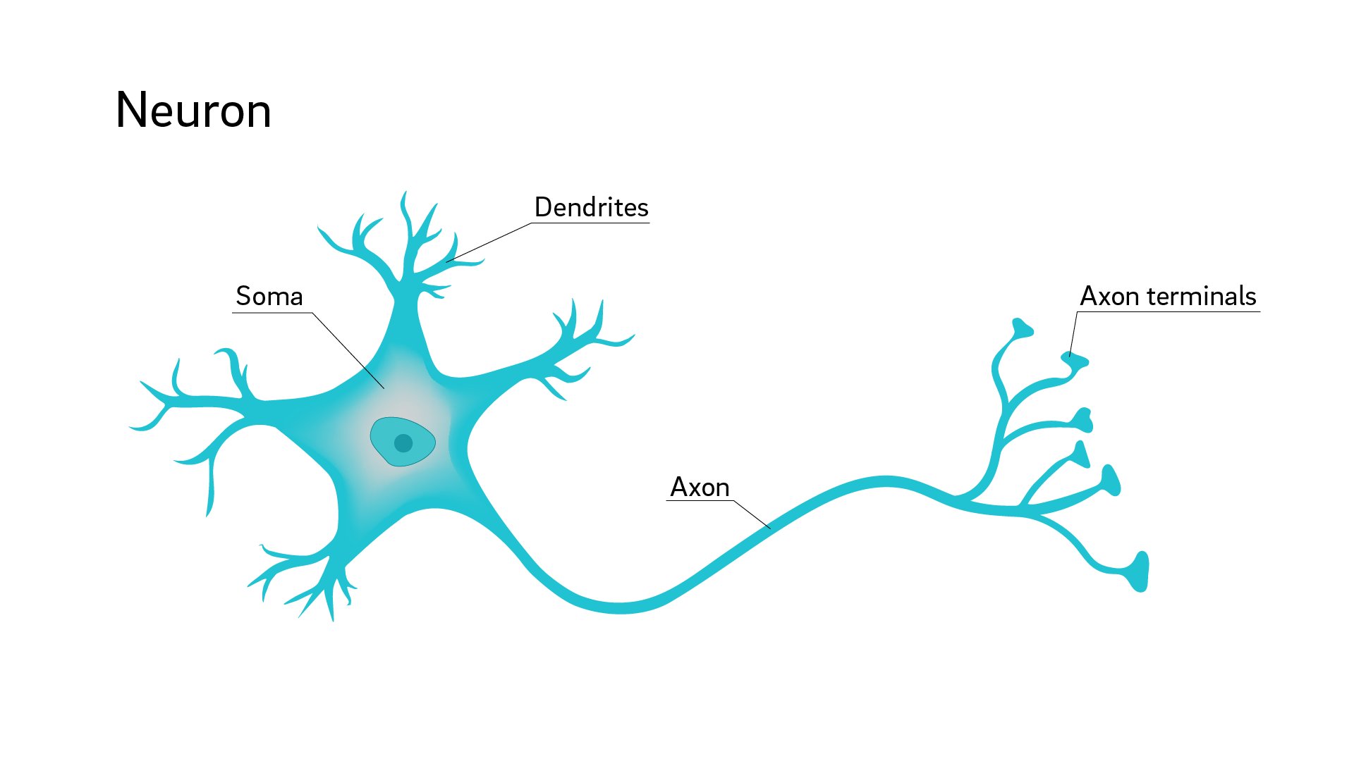

Neurons are interconnected in such a way that they have different functions, such as sensory neurons, which respond to such stimuli as sound, touch, or light; motor neurons, which control the muscle movements in the body; and interneurons, which are connected neurons within the same region of the brain or spinal cord.
神经元以这样的方式相互连接，它们具有不同的功能，如感觉神经元，对声音、触摸或光线等刺激作出反应；运动神经元，控制身体的肌肉运动；以及神经元间，是大脑或脊髓同一区域内的连接神经元。

3. Artificial Neural Networks (ANNs)

An artificial neural network tries to mimic the brain at its most basic level, i.e., that of the neuron.
人工神经网络试图模仿大脑最基本的层次，即神经元层次。
An artificial neuron has a similar structure to that of a human neuron and comprises the following sections.
人工神经元的结构与人类神经元类似，包括以下部分。
Input layer: This layer is similar to dendrites and takes input from other networks/neurons.
输入层： 该层类似于树突，接受来自其他网络/神经元的输入。接受来自其他网络/神经元的输入。
Summation layer: This layer functions like the soma of neurons. It aggregates the input signal received.
求和层： 该层的功能类似于神经元的体。它汇总接收到的输入信号。
Activation layer: This layer is also similar to a soma, and it takes the aggregated information and fires a signal only if the aggregated input crosses a certain threshold value. Otherwise, it does not fire.
激活层： 该层也类似于 “体”（soma），它接收汇总的信息，只有当汇总的输入超过一定的阈值时才发出信号。否则，它不会触发信号。
Output layer: This layer is similar to axon terminals in that it might be connected to other neurons/networks or act as a final output layer (for predictions).
输出层： 该层与轴突末端类似，可能与其他神经元/网络连接，或作为最终输出层（用于预测）。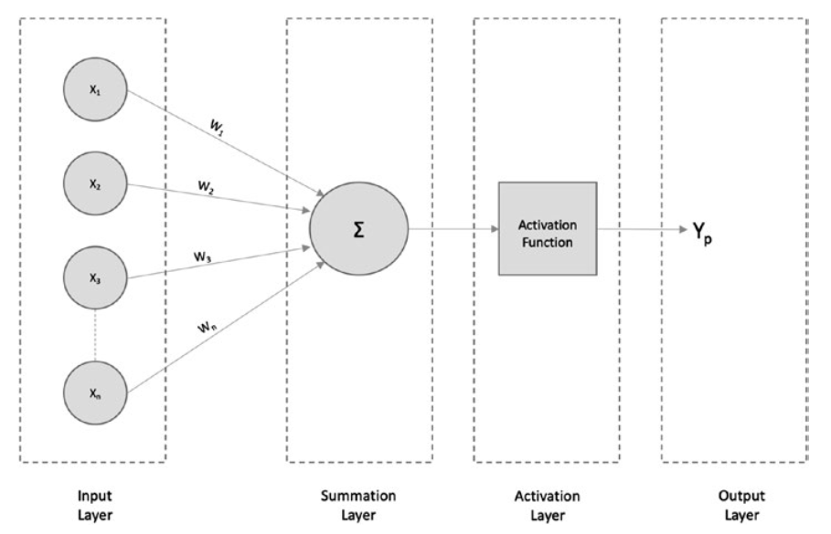

In the preceding figure, X ₁, X₂, X₃,…X_n are the inputs fed to the neural network.
在上图中，X1, X2, X3,…Xn 是神经网络的输入。
W₁, W₂, W₃,…Wn are the weights associated with the inputs, and Y is the final prediction.
W1、W2、W3,…Wn为与输入相关的权重，Y为最终预测值。
Many activation functions can be used in the activation layer, to convert all the linear details produced at the input and make the summation layer nonlinear.
激活层可使用多种激活函数，以转换输入端产生的所有线性细节，并使求和层成为非线性层。
This helps users acquire more details about the input data that would not be possible if this were a linear function.
这有助于用户获得输入数据的更多细节，而如果是线性函数则无法实现这一点。
Therefore, the activation layer plays an important role in predictions.
因此，激活层在预测中发挥着重要作用。
Some of the most familiar types of activation functions are sigmoid, ReLU, and softmax.
最常见的激活函数类型有sigmoid、ReLU和softmax。

4. Simple Neural Network Architecture

As shown in Figure, a typical neural network architecture is made up of an Input layer, Hidden layer, Output layer.
如图所示，典型的神经网络结构由输入层、隐藏层和输出层组成。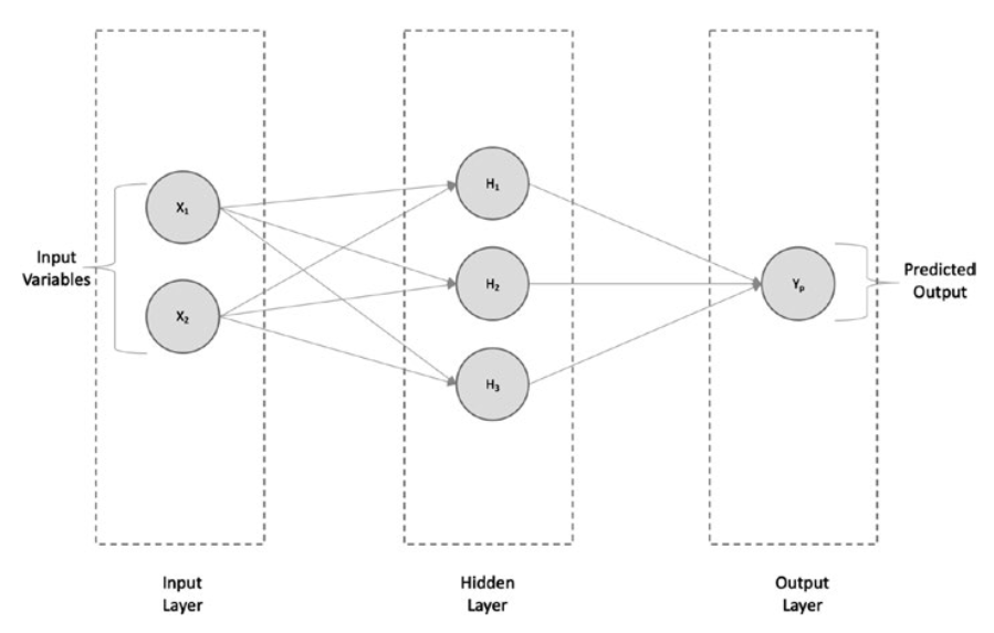

Simple neural network architecture—regression
简单的神经网络结构-回归
Every input is connected to every neuron of the hidden layer and, in turn, connected to the output layer.
每个输入都连接到隐层的每个神经元，然后再连接到输出层。
If we are solving a regression problem, the architecture looks like the one shown in Figure, in which we have the output Y_p, which is continuous if predicted at the output layer.
如果我们解决的是回归问题，则架构如图所示，其中我们有输出Yp，如果在输出层预测，则输出Yp是连续的。
If we are solving a classification (binary, in this case), we will have the outputs Yclass₁ and Y_class2, which are the probability values for each of the binary classes 1 and 2 at the output layer, as shown in Figure.
如果我们求解的是分类（本例中为二元分类），我们将得到输出Yclass1和Y class2，它们是输出层中二元分类1和2的概率值，如图所示。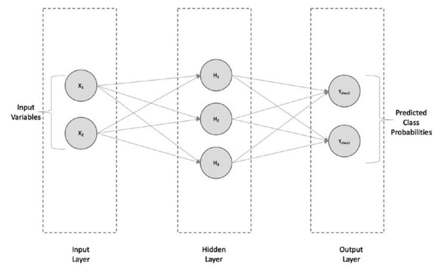

Simple neural network architecture—classification
简单神经网络架构-分类

5. Forward and Backward Propagation

In a fully connected neural network, when the inputs pass through the neurons (hidden layer to output layer), and the final value is calculated at the output layer, we say that the inputs have forward propagated.
在一个全连接的神经网络中，当输入通过神经元（从隐层到输出层），并在输出层计算出最终值时，我们称输入为前向传播。
Consider, for example, a fully connected neural network with two inputs, X₁ and X₂, and one hidden layer with three neurons and an output layer with a single output Y_p (numeric value).
例如，考虑一个全连接的神经网络，它有两个输入层X1和X2，一个有三个神经元的隐藏层和一个有单个输出Yp（数值）的输出层。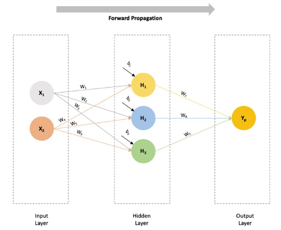

Forward propagation
前向传播
The inputs will be fed to each of the hidden layer neurons, by multiplying each input value with a weight (W) and summing them with a bias value (b).
通过将每个输入值与权值（W）相乘并与偏置值（b）相加，将输入输入到每个隐层神经元。
So, the equations at the neurons’ hidden layer will be as follows:
因此，神经元隐藏层的方程如下：
H₁ = W₁ * X₁ + W₄ * X ₂ + b₁
H₂ = W₂ * X₁ + W₅ * X ₂ + b₂
H₃ = W₃ * X₁ + W₆ * X ₂ + b₃
The values H₁, H₂, and H₃ will be passed to the output layer, with weights W₇, W₈, and W₉, respectively. The output layer will produce the final predicted value of Y_p.
值H₁、H₂和H₃将分别通过权重W₇、W₈和W₉传递给输出层。输出层将产生Y_p的最终预测值。
Y_p = W₇ * H₁ + W₈ * H₂ + W ₉ * H₃
As the input data (X₁ and X₂) in this network flows in a forward direction to produce the final outcome, Y_p, it is said to be a feed forward network, or, because the data is propagating in a forward manner, a forward propagation.
由于该网络中的输入数据（X₁和X₂）是向前流动的，从而产生最终结果Y_p，因此称其为前馈网络，或者，由于数据是向前传播的，因此称其为前向传播。
Now, suppose the actual value of the output is known (denoted by Y).
In this case, we can calculate the difference between the actual value and the predicted value, i.e., L = (Y - Y p )2, where L is the loss value.
在这种情况下，我们可以计算实际值与预测值之间的差值，即L = (Y - Y_p )²，其中L为损失值。
To minimize the loss value, we will try to optimize the weights accordingly, by taking a derivate of the loss function to the previous weights, as shown in Figure.
为了使损失值最小化，我们将尝试对权重进行相应的优化，将损失函数与之前的权重进行求导，如图所示。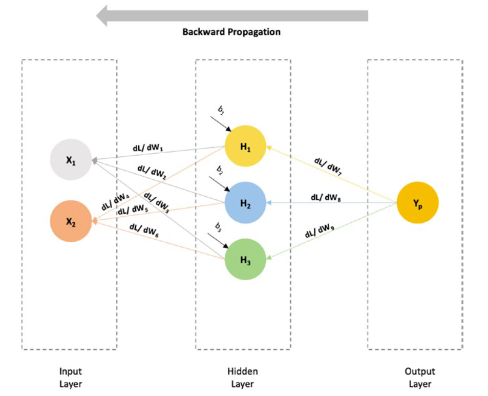

Backward propagation
反向传播
For example, if we have to find the rate of change of loss function as compared to W ₇, we would take a derivate of the Loss function to that of W₇ (d _L / d _{W7), and so on.
例如，如果我们需要求出与W7相比的损失函数变化率，我们将求出与W7相比的损失函数的导数（d L/d W7 ），以此类推。
As we can see from the preceding diagram, the process of taking the derivates is moving in a backward direction, that is, a backward propagation is occurring.
从上图可以看出，求导的过程是向后移动的，即发生了向后传播。
There are multiple optimizers available to perform backward propagation, such as stochastic gradient descent (SGD), AdaGrad, among others.
有多种优化器可用于执行反向传播，如随机梯度下降（SGD）、AdaGrad等。}

6. Building Neural Networks with TensorFlow 2.0

Using the Keras API with TensorFlow, we will be building a simple neural network with only one hidden layer.
利用Keras API和TensorFlow，我们将构建一个只有一个隐藏层的简单神经网络。

(1) About the Data Set

Let’s implement a simple neural network, using TensorFlow 2.0. For this, we will make use of the Fashion-MNIST data set by Zalando , which contains 70,000 images (in grayscale) in 10 different categories.
让我们使用TensorFlow 2.0实现一个简单的神经网络。为此，我们将使用Zalando提供的时尚-MNIST数据集，该数据集包含10个不同类别的7万张图片（灰度）。
The images are 28 × 28 pixels of individual articles of clothing, with values ranging from 0 to 255, as shown in Figure.
如图所示，图像为28×28像素的单件服装，数值范围为0至255。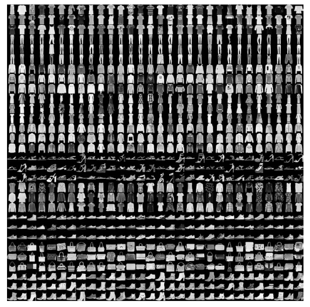

Sample from the Fashion-MNIST data set
(Source: https://bit.ly/2xqIwCH)
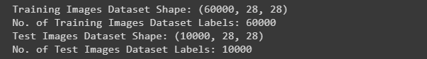
Of the total 70,000 images, 60,000 are used for training, and the remaining 10,000 images are used for testing.
在总共70,000幅图像中，60,000幅用于训练，其余10,000幅用于测试。
The labels are integer arrays ranging from 0 to 9.
标签为0至9的整数数组。
The class names are not part of the data set;
类名不属于数据集的一部分；
therefore, we must include the following mapping for training/prediction:
因此，我们必须包括以下训练/预测映射：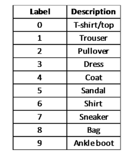

(Source: https://bit.ly/2xqIwCH)

# Create class_names list object for mapping labels to names
# 创建class_names列表对象，用于将标签映射为名称
class_names = ['T-shirt/top', 'Trouser', 'Pullover', 'Dress', 'Coat', 'Sandal', 'Shirt', 'Sneaker', 'Bag', 'Ankle boot']

# Use the below code to make sure that you select TensorFlow 2.0 in Colab
# 使用以下代码确保您在Colab中选择TensorFlow 2.0
try:
  %tensorflow_version 2.x
except Exception:
  pass

# Install necessary modules

from __future__ import absolute_import, division, print_function, unicode_literals

# Helper libraries
import numpy as np

# TensorFlow and tf.keras
import tensorflow as tf
from tensorflow import keras as ks

# Validating the TensorFlow version
print(tf.__version__)

# Load the Fashion MNIST dataset
# 加载时尚MNIST数据集
(training_images, training_labels), (test_images, test_labels) = ks.datasets.fashion_mnist.load_data()

1. 使用了ks.datasets.fashion_mnist.load_data()函数来加载数据集。这个函数会返回两个元组，分别表示训练集和测试集的图像数据以及对应的标签。
2. 训练集的图像数据保存在training_images变量中，训练集的标签保存在training_labels变量中。
3. 测试集的图像数据保存在test_images变量中，测试集的标签保存在test_labels变量中。

Data Exploration 数据分析

# Shape of Training and Test Set
#  训练集和测试集的形状
print('Training Images Dataset Shape: {}'.format(training_images.shape))
print('No. of Training Images Dataset Labels: {}'.format(len(training_labels)))
print('Test Images Dataset Shape: {}'.format(test_images.shape))
print('No. of Test Images Dataset Labels: {}'.format(len(test_labels)))

Data Preprocessing 数据预处理

As the pixel values range from 0 to 255, we have to scale these values to a range of 0 to 1 before feeding them to the model.
由于像素值的范围在 0 到 255 之间，因此在将这些值输入模型之前，我们必须将其缩放至 0 到 1 的范围。
We can scale these values (both for training and test datasets) by dividing the values by 255:
我们可以通过将这些值除以 255 来缩放这些值（包括训练数据集和测试数据集）：

training_images = training_images / 255.0

test_images = test_images / 255.0

1. 归一化通过将图像的像素值缩放到0到1的范围内，使得数据具有相同的尺度。
2. 代码中使用了除法运算符/，将训练集的图像数据training_images以及测试集的图像数据test_images都除以255.0。这是因为Fashion MNIST数据集中的像素值范围为0到255，除以255.0后可以将像素值缩放到0到1之间。

Model Building 模型训练

We will be using the keras implementation to build the different layers of a NN. We will keep it simple by having only 1 hidden layer.
我们将使用keras实现来构建NN的不同层。我们将保持简单，只有一个隐藏层。

input_data_shape = (28, 28)
hidden_activation_function = 'relu'
output_activation_function = 'softmax'

nn_model = ks.models.Sequential()
nn_model.add(ks.layers.Flatten(input_shape=input_data_shape, name='Input_layer'))
nn_model.add(ks.layers.Dense(32, activation=hidden_activation_function, name='Hidden_layer'))
nn_model.add(ks.layers.Dense(10, activation=output_activation_function, name='Output_layer'))

1. input_data_shape = (28, 28): 这行代码定义了输入数据的形状，即图像的大小为 28x28 像素。
2. hidden_activation_function = ‘relu’: 这行代码定义了隐藏层的激活函数，使用的是 ReLU 函数，它在神经网络中常用于引入非线性。
3. output_activation_function = ‘softmax’: 这行代码定义了输出层的激活函数，使用的是 Softmax 函数，它通常用于多类别分类问题，将输出转化为概率分布。
4. nn_model = ks.models.Sequential(): 这行代码创建了一个 Sequential 模型对象，它是 Keras 中的一种基本模型类型，可以按顺序添加各个层。
5. nn_model.add(ks.layers.Flatten(input_shape=input_data_shape, name=‘Input_layer’)): 这行代码添加了一个 Flatten 层作为输入层，用于将输入数据从二维形状（28x28）展平为一维向量。
6. nn_model.add(ks.layers.Dense(32, activation=hidden_activation_function, name=‘Hidden_layer’)): 这行代码添加了一个全连接层作为隐藏层，包含 32 个神经元，并使用 ReLU 激活函数。
7. nn_model.add(ks.layers.Dense(10, activation=output_activation_function, name=‘Output_layer’)): 这行代码添加了一个全连接层作为输出层，包含 10 个神经元（假设是一个 10 类别的分类问题），并使用 Softmax 激活函数。

nn_model.summary()

运行结果：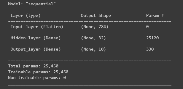

1. nn_model.summary() 是用于打印神经网络模型的摘要信息。
2. 模型的总体结构：显示每个层的名称、输出形状和参数数量。
3. 每个层的输出形状：显示每个层的输出张量形状。
4. 可训练参数的总数：显示模型中所有可训练参数的总数量。

Now, we will use an optimization function with the help of compile method.
现在，我们将在编译方法的帮助下使用优化函数。
An Adam optimizer with objective function as sparse_categorical_crossentropy which optimzes for the accuracy metric can be built as follows:
Adam优化器的目标函数为sparse_categorical_crossentropy，其优化精度指标如下：

optimizer = 'adam'
loss_function = 'sparse_categorical_crossentropy'
metric = ['accuracy']
nn_model.compile(optimizer=optimizer, loss=loss_function, metrics=metric)

1. optimizer = ‘adam’：这行代码将字符串值’adam’赋给变量optimizer。在这种情况下，'adam’表示Adam优化算法，它是训练深度学习模型的常用选择。
2. loss_function = ‘sparse_categorical_crossentropy’：这行代码将字符串值’sparse_categorical_crossentropy’赋给变量loss_function。这个损失函数通常用于多类别分类问题，其中目标标签是整数。
3. metric = [‘accuracy’]：这行代码将包含字符串’accuracy’的列表赋给变量metric。准确率指标是分类任务中常用的评估指标，用于衡量正确预测标签的百分比。
4. nn_model.compile(optimizer=optimizer, loss=loss_function, metrics=metric)：这行代码使用指定的优化器、损失函数和指标编译神经网络模型nn_model。compile()函数配置模型进行训练，指定优化算法、训练过程中要最小化的损失函数以及用于评估模型性能的指标。

nn_model.fit(training_images, training_labels, epochs=10)

运行结果：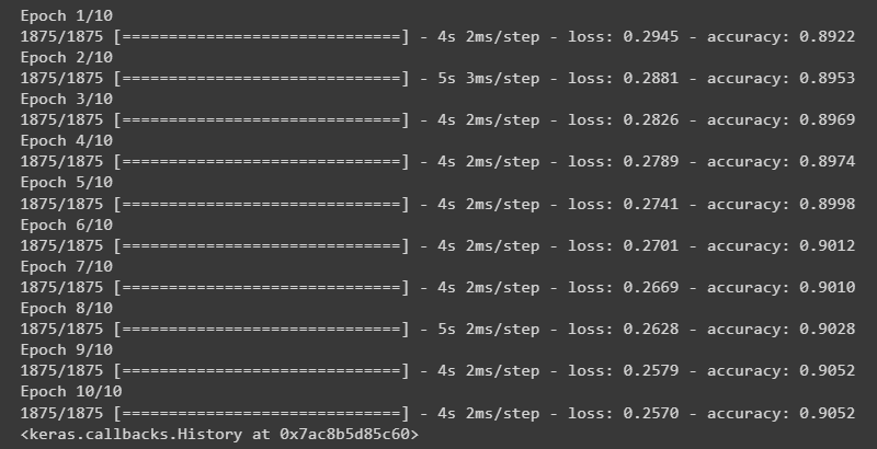

Model Evaluation 模型评估

Training Evaluation 训练评估

training_loss, training_accuracy = nn_model.evaluate(training_images, training_labels)

print('Training Data Accuracy {}'.format(round(float(training_accuracy),2)))

运行结果：

1. nn_model.evaluate(training_images, training_labels)：这行代码调用了神经网络模型的evaluate方法，用于评估模型在给定的训练数据集上的性能。training_images是训练图像数据，training_labels是对应的训练标签。
2. training_loss, training_accuracy = nn_model.evaluate(training_images, training_labels)：这行代码将evaluate方法返回的结果分别赋值给training_loss和training_accuracy两个变量。training_loss表示模型在训练数据集上的损失值，training_accuracy表示模型在训练数据集上的准确率。
3. print(‘Training Data Accuracy {}’.format(round(float(training_accuracy),2)))：这行代码打印输出了训练数据集的准确率。使用format方法将字符串中的占位符{}替换为round(float(training_accuracy),2)的值，即将training_accuracy转换为浮点数并保留两位小数。最终输出的字符串形式为"Training Data Accuracy X.XX"，其中X.XX表示训练数据集的准确率。

Test Evaluation 测试评估

test_loss, test_accuracy = nn_model.evaluate(test_images, test_labels)

print('Test Data Accuracy {}'.format(round(float(test_accuracy),2)))

运行结果：

1. nn_model.evaluate(test_images, test_labels)会使用测试图像和标签作为输入，计算模型在测试数据集上的损失值和准确率。
2. 返回值test_loss和test_accuracy分别表示模型在测试数据集上的损失值和准确率。
3. print(‘Test Data Accuracy {}’.format(round(float(test_accuracy),2)))将测试数据集的准确率打印出来，并使用format函数将准确率格式化为浮点数，并保留两位小数。

7. Deep Neural Networks (DNNs)

When a simple neural network has more than one hidden layer, it is known as a deep neural network (DNN). Figure shows the architecture of a typical DNN.
当一个简单的神经网络有一个以上的隐藏层时，它被称为深度神经网络（DNN）。图显示了典型DNN的结构。

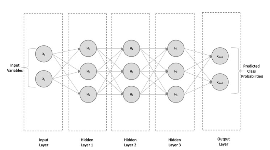
Deep neural network with three hidden layers
具有三个隐藏层的深度神经网络
It consists of an input layer with two input variables, three hidden layers with three neurons each, and an output layer (consisting either of a single output for regression or multiple outputs for classification).
它由一个包含两个输入变量的输入层、三个各包含三个神经元的隐藏层和一个输出层（在回归时由单个输出组成，在分类时由多个输出组成）组成。
The more hidden layers, the more neurons. Hence, the neural network is able to learn the nonlinear (non-convex) relation between the inputs and output.
隐藏层越多，神经元就越多。因此，神经网络能够学习输入和输出之间的非线性（非凸）关系。
However, having more hidden layers adds to the computation cost, so one has to think in terms of a trade-off between computation cost and accuracy.
然而，增加隐藏层会增加计算成本，因此必须在计算成本和准确性之间进行权衡。

8. Building DNNs with TensorFlow 2.0

We will be using the Keras implementation to build a DNN with three hidden layers.
我们将使用Keras实现来构建具有三个隐藏层的DNN。
The steps in the previous implementation of a simple neural network, up to the scaling part, is same for building the DNN.
前面实现简单神经网络的步骤，直到缩放部分，与构建DNN的步骤相同。
Therefore, we will skip those steps and start directly with building the input and hidden and output layers of the DNN, as follows:
因此，我们将跳过这些步骤，直接开始构建 DNN 的输入层、隐藏层和输出层，如下所示：

input_data_shape = (28, 28)
hidden_activation_function = 'relu'
output_activation_function = 'softmax'

dnn_model = ks.models.Sequential()
dnn_model.add(ks.layers.Flatten(input_shape=input_data_shape, name='Input_layer'))
dnn_model.add(ks.layers.Dense(256, activation=hidden_activation_function, name='Hidden_layer_1'))
dnn_model.add(ks.layers.Dense(192, activation=hidden_activation_function, name='Hidden_layer_2'))
dnn_model.add(ks.layers.Dense(128, activation=hidden_activation_function, name='Hidden_layer_3'))
dnn_model.add(ks.layers.Dense(10, activation=output_activation_function, name='Output_layer'))

dnn_model.summary()

运行结果：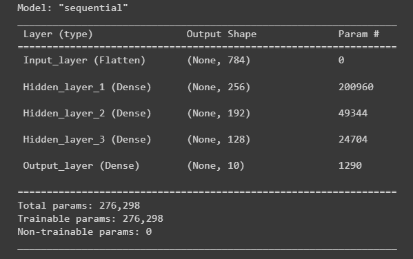

Now, we will use an optimization function with the help of the compile method.
现在，我们将在编译方法的帮助下使用优化函数。
An Adam optimizer with the objective function sparse_ categorical_crossentropy, which optimizes for the accuracy metric, can be built as follows:
Adam优化器的目标函数为sparse_ categorical_crossentropy，该优化器对准确度指标进行优化，可构建如下：

optimizer = 'adam'
loss_function = 'sparse_categorical_crossentropy'
metric = ['accuracy']
dnn_model.compile(optimizer=optimizer, loss=loss_function, metrics=metric)

dnn_model.fit(training_images, training_labels, epochs=20)

运行结果：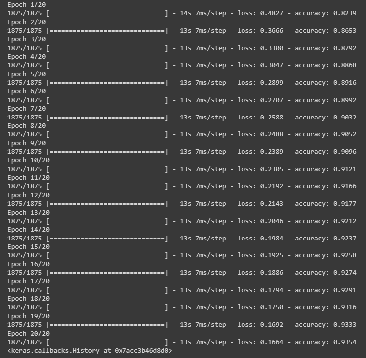

Model Evaluation

Training Evaluation

training_loss, training_accuracy = dnn_model.evaluate(training_images, training_labels)

print('Training Data Accuracy {}'.format(round(float(training_accuracy),2)))

运行结果：

Test Evaluation

test_loss, test_accuracy = dnn_model.evaluate(test_images, test_labels)

print('Test Data Accuracy {}'.format(round(float(test_accuracy),2)))

运行结果：

As observed, the training accuracy for the simple neural network is about 90%, whereas it is 94% for the DNNs, and the test accuracy for the simple neural network is about 87%, whereas it is 89% for DNNs.
据观察，简单神经网络的训练精度约为90%，而DNN的训练精度为94%；简单神经网络的测试精度约为87%，而DNN的测试精度为89%。
It goes to show that we were able to achieve higher accuracy by adding more hidden layers to the neural network architecture.
这表明，通过在神经网络结构中增加更多的隐藏层，我们能够获得更高的精度。

9. Estimators Using the Keras Model

We built various machine learning models, using premade estimators.
我们使用预制估计器建立了各种机器学习模型。
However, the TensorFlow API also provides enough flexibility for us to build custom estimators.
然而，TensorFlow API也为我们提供了足够的灵活性来构建自定义估算器。
In this section, you will see how we can create a custom estimator, using a Keras model.
在本节中，您将看到我们如何使用 Keras 模型创建自定义估算器。
The implementation follows.
具体实施如下。
Let’s start by loading the necessary modules.
首先加载必要的模块。

Import the required Modules

from __future__ import absolute_import, division, print_function, unicode_literals
import numpy as np
import pandas as pd
import tensorflow as tf
from tensorflow import keras as ks
import tensorflow_datasets as tf_ds

print(tf.__version__)

Now, create a function to load the iris data set.

现在，创建一个函数来加载鸢尾花数据集。

def data_input():
  train_test_split = tf_ds.Split.TRAIN
  iris_dataset = tf_ds.load('iris', split=train_test_split, as_supervised=True)
  iris_dataset = iris_dataset.map(lambda features, labels: ({'dense_input':features}, labels))
  iris_dataset = iris_dataset.batch(32).repeat()
  return iris_dataset

Build a simple Keras model.

activation_function = 'relu'
input_shape = (4,)
dropout = 0.2
output_activation_function = 'sigmoid'

keras_model = ks.models.Sequential([ks.layers.Dense(16, activation=activation_function, input_shape=input_shape), ks.layers.Dropout(dropout), ks.layers.Dense(1, activation=output_activation_function)])

Now, we will use an optimization function with the help of the compile method. An Adam optimizer with the loss function categorical_crossentropy can be built as follows:

现在，我们将在编译方法的帮助下使用一个优化函数。一个具有损失函数categorical_crossentropy的Adam优化器可以如下建立：

loss_function = 'categorical_crossentropy'
optimizer = 'adam'

keras_model.compile(loss=loss_function, optimizer=optimizer)
keras_model.summary()

运行结果：

Build the estimator, using tf.keras.estimator.model_to_estimator:

使用tf.keras.estimator.model_to_estimator构建估计器：

model_path = "/keras_estimator/"
estimator_keras_model = ks.estimator.model_to_estimator(keras_model=keras_model, model_dir=model_path)

Train and evaluate the model.

estimator_keras_model.train(input_fn=data_input, steps=25)
evaluation_result = estimator_keras_model.evaluate(input_fn=data_input, steps=10)
print('Fianl evaluation result: {}'.format(evaluation_result))

运行结果：

10. Conclusion

In this chapter, you have seen how easy it is to build neural networks in TensorFlow 2.0 and also how to leverage Keras models, to build custom TensorFlow estimators.
在本章中，您将看到在TensorFlow 2.0中构建神经网络是多么容易，以及如何利用Keras模型构建自定义TensorFlow估计器。